For many of us, life as we now know it would be almost impossible without Google Drive. Of course, Microsoft Office loyalists will disagree and justifiably so. However, with work from home becoming a norm and professionals having to make the shift to Google Sheets, Docs, and practically everything Drive related, whether willingly or not, we must make the move now.
This brings us to the subject of the article, i.e, how to make a histogram on Google Sheets. We suspect the reason you’re here is that you’ve realized/discovered that things work a little differently on Google Sheets as compared to the way they did with Excel or whichever software you used before for number crunching and analyzing data. One thing you can be assured of is that Google Sheets is very easy to use and navigate. Just focus on letting go of Excel tendencies and this tutorial will do the rest for you. Let’s dive in!
Related: How to get Bitmoji in Google Classroom
How to construct a Histogram chart/graph
The premise is more or less the same with Google Sheets just like it was for Excel. You need to apply the relevant cell formula to manipulate data and calculate numbers if you want your chart to be really thorough. The next steps will elaborate on how to add a Histogram chart.
Create a data range
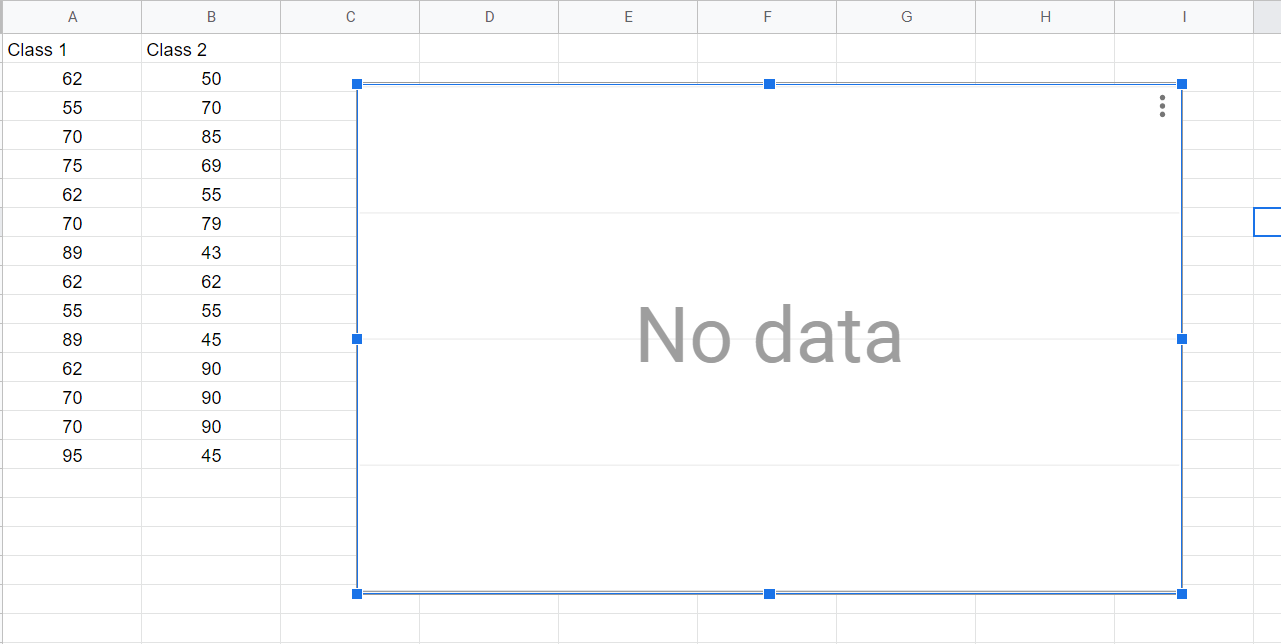
A data range is basically a cell grid that you create with relevant numeric information that is to be represented on the Histogram. For the purpose of this article, we’ve created two data cells ranging between values 43 and 95. Here’s a look at our data range allocated to columns A and B.
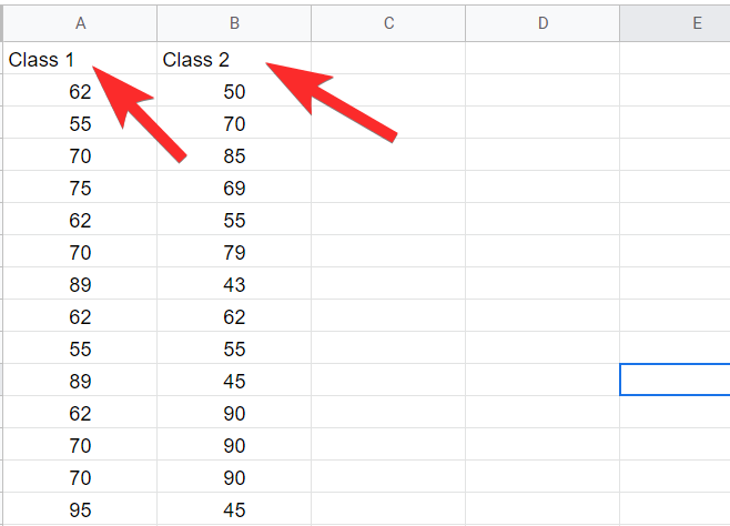
We will be using these columns to create our Histogram. You can create your Histogram using this one or use data of your own.
Related: How to use Google Meet in Google Classroom
How to add a Histogram Chart
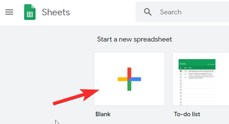
First, open a blank spreadsheet in Google Sheets by clicking the blank icon.
 You will now be looking at a blank spreadsheet. From the menu panel, click on Insert.
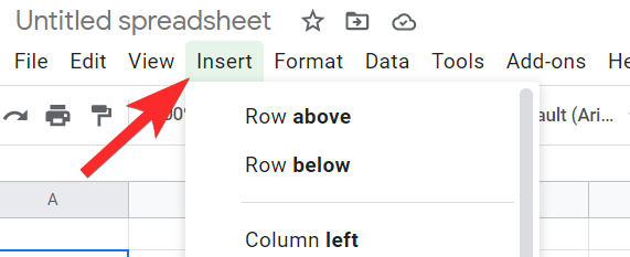
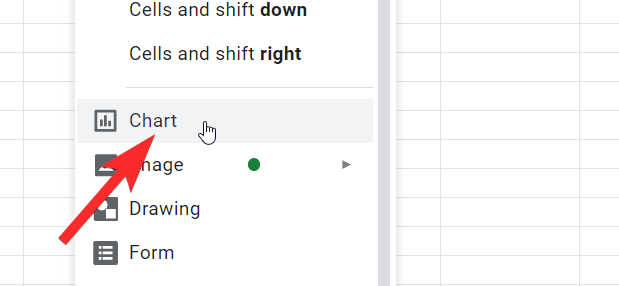
From the menu that opens, click on Chart.
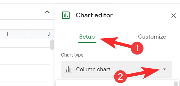
Now you will see a Chart editor open next towards the right side. From the Setup tab, click on the dropdown menu for Chart Type.
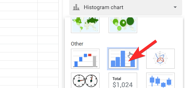
Scroll towards the end of the menu till you reach the Other option where you will see an option for Histogram chart, click on it.
Great! The histogram chart has now been added to your sheet. It should look similar to this image:
Related: 16 cool Google Meet Ideas for Teachers
How to edit the Histogram chart- Setup Tab
The Setup Tab is where you will find the options and settings that are required to add the relevant information from the columns to the chart. This is where you set the base for the histogram. Basically, the Setup Tab allows you to incorporate the data sets into it.
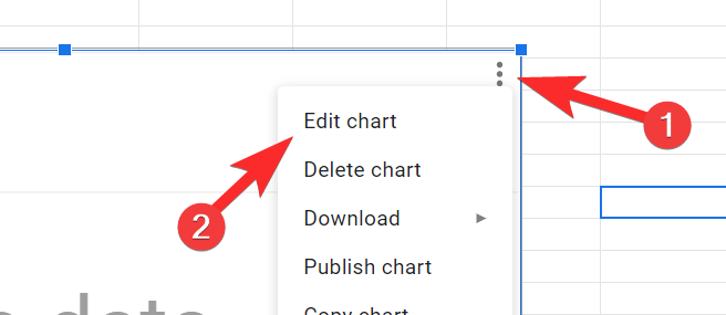
For any kind of editing activity, you will have to click on the three-dot menu icon on the top right section of the chart and then click on select the Edit chart option.
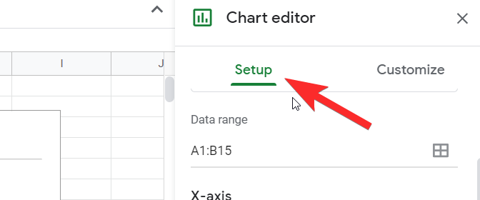
Once you do, the Chart Editor will pop up towards the right side of the screen. Here you will see two tabs, Setup and Customize. Click on Setup.
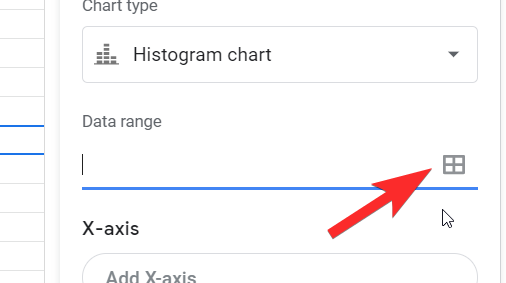
Within the Setup tab in the Chart Editor, you have to set the data range for the chart. To do this, click on the Select Data Range icon.
Now, you can choose one of two formats. Either club both the columns together to form a single panel chart. In which case add all the cells (A1: B15) in one range.
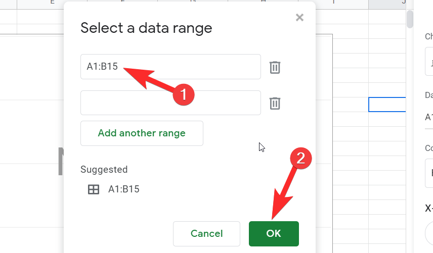
Or, you can create another range for the next column as well.

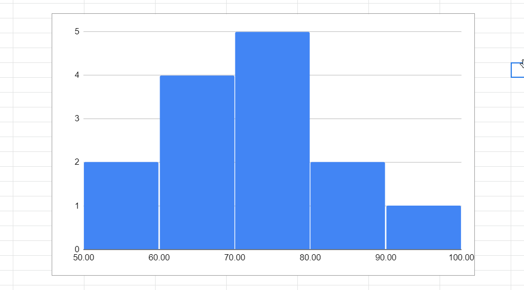
In any case, your Histogram will look like this:
In the Series section, you can create one entire set of series which would then be A1:B15 or you can also separate the two columns.
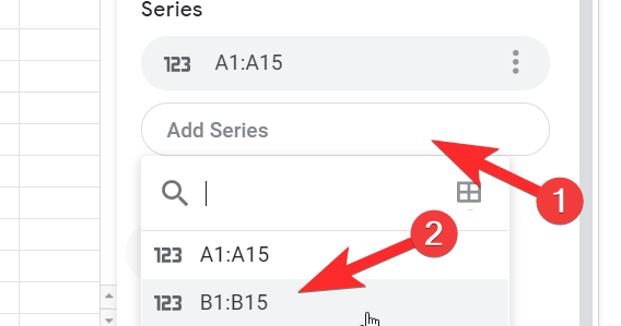
In which case your Histogram will look like this:

If you choose to club all the columns into one series, then the histogram chart won’t look and different from what it did before.
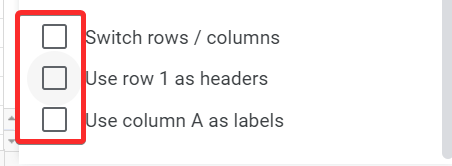
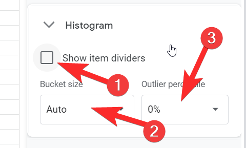
Finally, in the last section of the Setup Tab, you will see the following options with checkboxes. You can select them if you wish to incorporate those settings in the chart.
Great! now that you have set up your histogram, let’s look at how you can customize it.
Related: Google Meet for Teachers: A Complete Tutorial and 8 Useful Tips
How to edit the Histogram chart- Customize Tab
In the customize tab, you can change the look and feel as well as add features to your histogram.

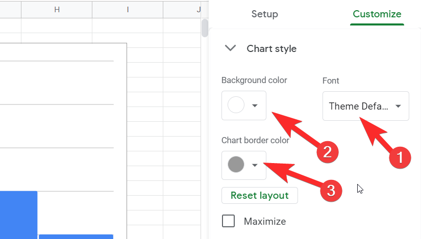
Let’s look at each section in the Customize Tab starting with Chart Style.
In the Chart Style section, you change the font, background, and chart border color of the chart.
Next, you can set the bucket size of the chart in case you want to increase it. Sheets offers a bucket size of up to 50. You can also show the x-axis in outliers.
In the next section, you can name your chart and change the font and font size.
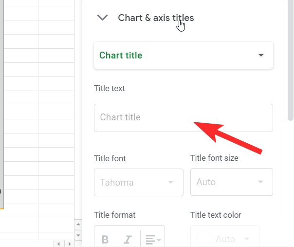
When you click on the chart title, you can name every axis and give subtitles should you wish.

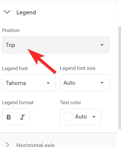
You can even set the position of the legend.
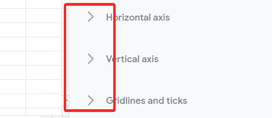
The next sections will allow you to customize the font of the text that represents both the axis. You can choose to forgo this unless you have to follow a design guideline. The same applies to gridlines and ticks. Simply click on the arrow for each section to open them and apply whichever settings you want.
When customized, our histogram came out looking like the image below. We’re
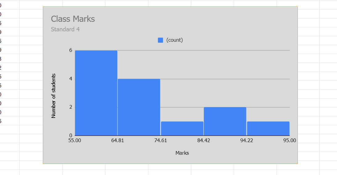
There you go! You now know how to create a histogram graph on Google Sheets. Let us know what you want to learn next. Take care and stay safe.
RELATED: