Excel sheets have always been the staple of huge data sets. They allow you to manage various entries easily and automatically while making sure that you can use functions, formulas, and all other features offered by spreadsheets.
Although great in their regard, spreadsheets can’t prevent you from having duplicate entries. This means that you will have to manually find and take care of them on your own whenever necessary.
While removing duplicates in Google Sheets is easy, what about highlighting them? Let’s find out!
How to highlight duplicates in Google Sheets: Step-by-step guide with pictures
We will be using conditional formatting to our advantage, to find and highlight duplicates in Google Sheets.
Follow either of the guides below depending on your current device and requirements.
Method 1: Use Conditional formatting on desktop devices
Conditional formatting allows you to apply formatting to certain cells containing data relevant to the formula defined by you.
You can use this to your advantage, to find and apply highlight only to duplicate cells in your current Sheet.
Follow either of the guides below to help you along with the process.
COUNTIF is the formula that we will be using to highlight duplicates in our Sheet. Follow one of the sections below depending on the range of your data.
1.1 For a single column
If you wish to highlight duplicates in a single column then you can use the formula given below. Follow the subsequent steps to help you along with the process.
=COUNTIF(M:M,M1)>1
M:M is your range here while M1 is the criterion. If you’re familiar with formulas, then you can copy-paste and use the formula above in your Google Sheet. If not, then start by navigating to the concerned sheet.

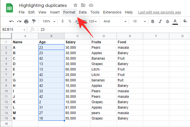
Use the Shift key on your keyboard or the column label at the top to select the column where you wish to search for duplicates.

Now click on ‘Format’ at the top in your toolbar.
Click and select ‘Conditional formatting’.

Your selected range will now be automatically added to the conditional formatting sidebar on your left. Click on the next drop-down menu for ‘Formula rules’ and select ‘Custom formula is’.

Now copy-paste the formula in the new space. You can also use the one linked below for convenience.
=COUNTIF(M:M,M1)>1

Replace M with the first cell of your range and subsequently the next one with the last cell in your range. The rest of the formula does not need editing and highlights should now be applied to duplicates on your left.

You can change the highlight/fill color for duplicate cells by using the picker in your sidebar.

Click on ‘Done’ to finalize and save your rule.

And that’s it! That’s how you can select duplicates in a particular column in Google Sheets.
1.2 For multiple columns
If you wish to find and highlight duplicate cells in multiple columns then you can use the guide mentioned below instead. Let’s get started!
Open the concerned sheet and select multiple columns in your sheet where you wish to identify and highlight duplicates. You can either click and drag on your screen or use the keyboard. You can also choose to manually define your range and skip this step entirely.

Click on ‘Format’ in your toolbar at the top.

Select ‘Conditional formatting’.

Now click on the drop-down menu and select ‘Custom formula is’.

Type in your desired formula in the following syntax
=COUNTIF(M$1:N$1,O1)>1
Replace M & N with the cell number of your desired columns. Similarly, replace O1 with your criteria for finding duplicates.

The duplicates will now be automatically highlighted in the default color.

You can change the same by clicking on the picker in the toolbar at the bottom.

And that’s it! You will now have highlighted duplicates in multiple columns in your Google Sheet.
Tips to search in multiple columns
Google Sheets uses the $ symbol to define absolute columns and rows. This means that if you wish to highlight duplicates from a single column value or multiple column values then this symbol can come in handy.
Keep in mind, you will need to use this before the range value to define the absolute column. Use the example below for further reference.
=COUNTIF(M$1:P$1,$O1)>1
The example above will find us duplicates from the given range based on the absolute values contained in the O column.
Method 2: Use Conditional Formatting on Android
You can also use conditional formatting on Android devices. Follow the guide below to apply conditional formatting to a Sheet to highlight duplicate entries.
2.1 For a single column
Open the Google Sheets app on your device and tap on a cell to select it.

Now drag one of the corners to select your desired range.

Once you have selected the range, tap on the ‘Format options’ icon at the top.

Scroll down and tap on ‘Conditional formatting’.

Tap on ‘Add’ in the top right corner.

The selected range will now be automatically entered for you. Tap on the drop-down menu and select ‘Custom rule is’.

Now use the following formula to find duplicates in the selected range.
=COUNTIF(M1:M10,M1)>1

Replace M1 with the address of the first cell in your column and subsequently M10 with the address of the last cell in the selected column. Replace M1 with your desired criterion, but we recommend setting it to the first cell of your column unless dealing with blank cells. Choose your formatting style by tapping on one of the presets.

You can also set a custom style by tapping on ‘+’.

Once you are done, tap on ‘Save’ in the top right corner.

Use the back gesture to go back to the selected Sheet if needed and the conditional formatting should now be already applied to the selected range. You can now continue finding duplicates in other columns and rows.
2.2 For multiple columns
You can use the following syntax when searching multiple columns for duplicates. This is the same as the formula used on desktop devices and if you need any help running the same, you can use the guide above to help you along with the process.
=COUNTIF(M$1:N$1,O1)>1
As usual, replace M$1 with the first cell of your range and N$1 with the last cell of your range. Ensure that you preserve the $ symbol to define absolutes.
Lastly, replace O1 with a criterion of your own depending on the data set you are assessing.
How to remove duplicates in Google Sheets
Now that you’ve found your duplicates, do you wish to remove them? Here’s how you can do that in Google Sheets.
Open Google Sheets and select the desired range from where you wish to remove duplicates.

Now click on ‘Data’ in your toolbar at the top.

Click and select ‘Data cleanup’.

Now click on ‘Remove duplicates’.

Check the box for ‘Select all’ and the respective columns in your range. This also gives you the choice of selectively excluding certain columns from this process.

Once you have made your choice, click on ‘Remove duplicates’.

The duplicates will now be removed from the selected column. Click on ‘Ok’ to save your changes and continue editing the Sheet as needed.

FAQs
Here are a few commonly asked questions about highlighting duplicates in Google Sheets that should help get you up to speed with the latest information.
Troubleshoot your results
If you’re new to using conditional formatting and formulas in Google Sheets then it can be quite intimidating, especially if your formulas are unable to show you the intended results.
Here are a couple of things you should check to troubleshoot your results when trying to highlight duplicates in Google Sheets.
- Check your Range
- Check absolute values
- Check your criterion
COUNTIFandUNIQUEvariables are not case sensitive.- Ensure the data in cells is supported for conditional formatting
- Check for missed spaces
- Check for incorrect syntax
Can you use conditional formatting on iOS devices?
Unfortunately, Google apps usually have limited support for iOS devices, and this is the case with Google Sheets as well. You can not use conditional formatting in the Google Sheets app for iOS.
We recommend you switch to a desktop device or use a chromium-based mobile browser to force the desktop website for Google Sheets on your mobile device.
You might have to try a few browsers to find one that works the best with scaling.
Can you highlight unique items instead?
No, Unfortunately, the UNIQUE formula is currently unsupported by conditional formatting which means that you can not use it to highlight unique items. You can only use it to get results in an empty cell/column.
What if you are looking for data that repeats 3 or 4 times?
In the syntax for COUNTIF, we use the > symbol to define how many times a data set is repeating in the selected range. Thus if you wish to find entries repeating thrice or even four times, you can replace 1 with the desired number.
As an example, if you’re looking for entries in the B column that repeat four times for the first 100 rows, then you will use the following syntax.
=COUNTIF(B1:B100,B1)>4

Note: The result will also include entries that repeat more than 4 times in the selected range as well.
We hope this post helped you highlight duplicates in Google Sheets. If you face any issues or have any more questions for us, feel free to reach out using the comments section below.
RELATED: