Excel is one of the most prominent spreadsheet management tools currently available on the market. It offers tons of functions, view options, and even variables to manage all your business data in one place. If you have been using Excel for a while then you might be familiar with its complexity especially if you have data that amounts to hundreds of rows and columns. This can make it quite difficult for you to keep track of the necessary categories or important data in certain columns and rows that you wish to verify.
Thankfully, Excel allows you to freeze such data so that it is always visible on your screen no matter where you scroll in the spreadsheet. Let’s take a quick look at this functionality.
What is the ‘Freeze panes’ option in Excel?
Freeze panes is a term in Excel used to denote static columns and rows. These rows and columns can be manually selected and turned into static elements. This ensures that the data in these rows and columns are always visible on your screen regardless of the currently selected cell, row, or column in the spreadsheet.
This functionality helps with better viewing of data, emphasizing categories, verifying data, corroboration against other readings, and much more.
How to freeze panes in Excel
When it comes to freezing panes in Excel you get 3 options; you can either freeze rows, columns, or a collection of rows and columns. Follow one of the guides below that best fits your needs.
Freeze Rows
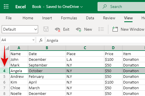
Open the concerned Spreadsheet and find the rows you wish to freeze. Once found, click and select the row beneath your selected rows by clicking on its number on the left side.
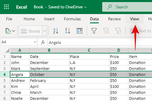
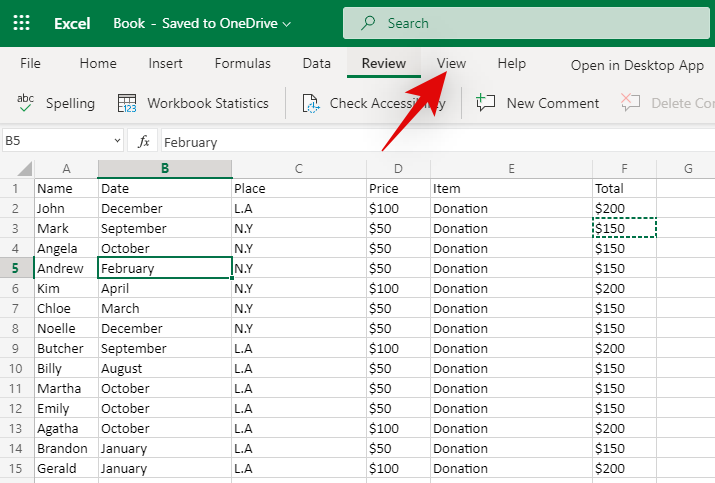
Once selected, click on ‘View’ at the top of your screen.
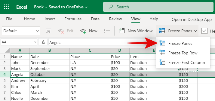
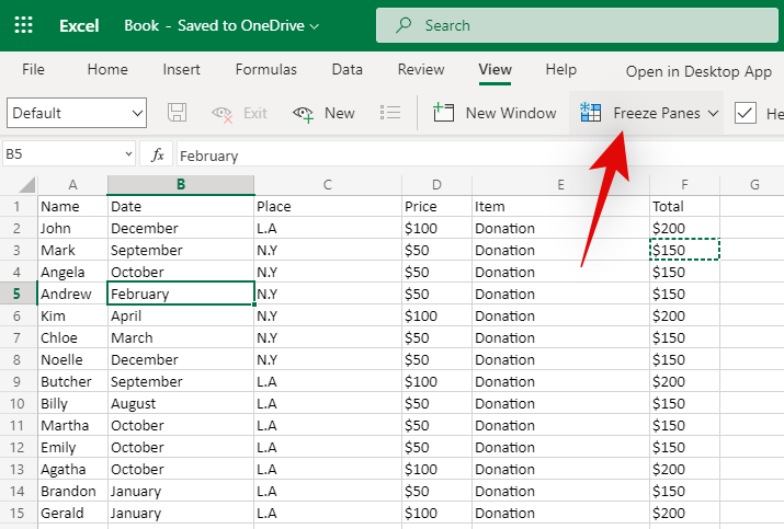
Now click on ‘Freeze Panes’.

Finally, select ‘Freeze Panes’
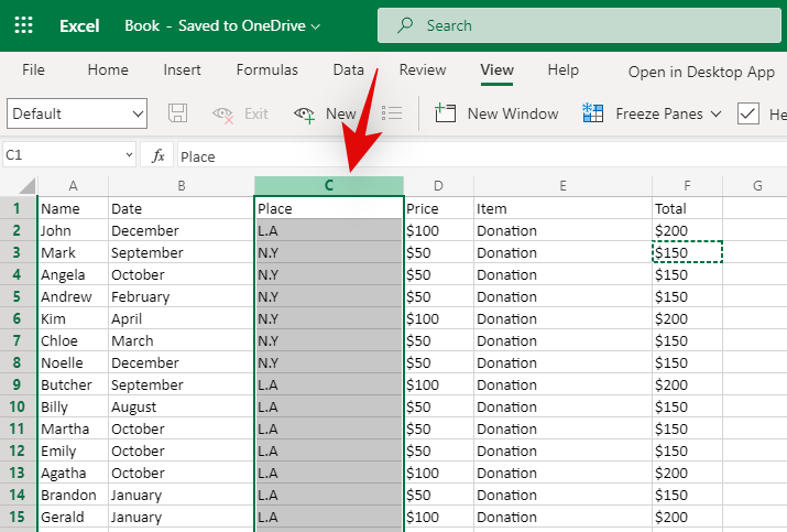
And that’s it! All the rows above your selected row will now be frozen and static on your screen. They will always be visible regardless of your position in the spreadsheet.
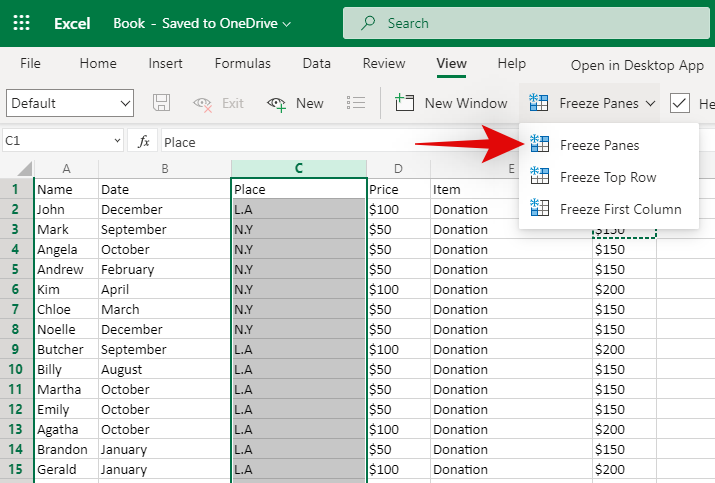
Freeze Columns
Open a spreadsheet and find all the columns you wish to freeze. Now click and select the entire column to the right of your selection.
Click on ‘View’ at the top of your screen.

Now select ‘Freeze Panes’.

Click on ‘Freeze Panes’ to freeze all the columns to the left of your selection.
And that’s it! All the concerned columns should now be frozen in the spreadsheet. They will remain static no matter how far you scroll horizontally.
Freeze Rows & Columns
Find the rows and columns you wish to freeze. Now select the cell beneath the intersection of your selection. For example, if you wish to select columns A, B, and C, and row 1, 2, and 3, then you need to select cell D4. This would be the intersection point for your chosen rows and columns.

Once selected, click on ‘View’ at the top of your screen.
Now click on ‘Freeze panes’.
Click on ‘Freeze panes’ again to freeze the rows and columns around your selected cell.
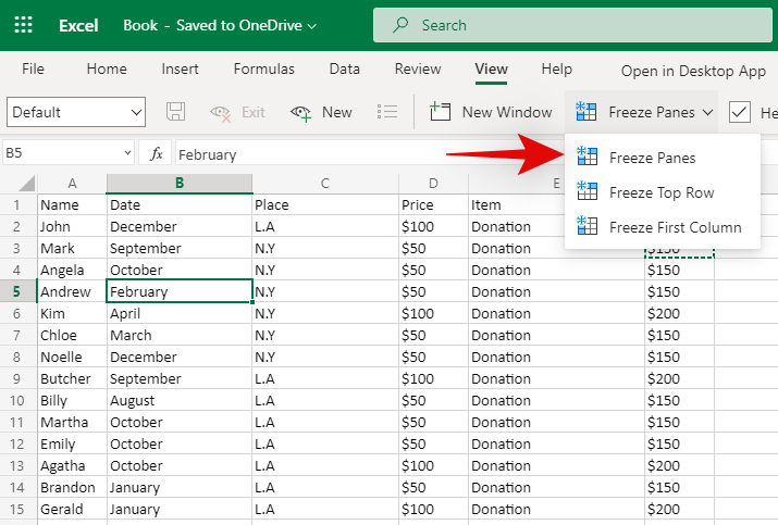
And that’s it! Your selected rows and columns should now be frozen in the concerned spreadsheet.
I hope you were easily able to freeze panes using the guide above. If you have any more questions, feel free to reach out using the comments section below.