
Adding axis labels to your charts in Google Sheets is easy, and you can do it on your PC (using the Google Sheets website) or phone (using the Google Sheets app). Find the step-by-step guides to add a vertical axis label or horizontal axis label for both types of devices below.
Add axis labels in Google Sheets on a computer
Use the guide below to add a vertical axis label or horizontal axis label to your chart in a Google Sheets document easily using your computer.
Step 1: Open a web browser of your choice, visit the Google Sheets website (docs.google.com/spreadsheets/u/0/), and then open the Google Sheets document in which you have the chart you want to add axis labels in.

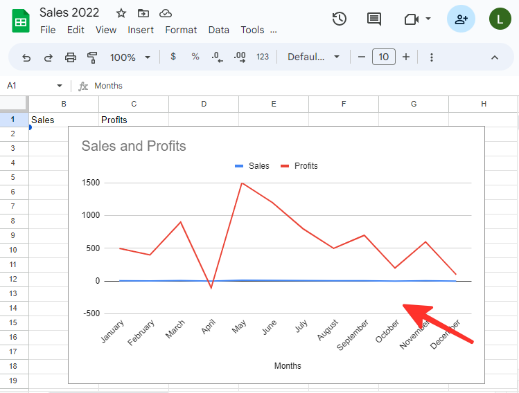
Step 2: To add axis labels to a chart, simply double-click on the chart itself. You can double-click on any part of the chart.
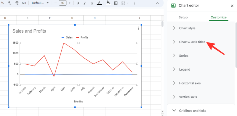
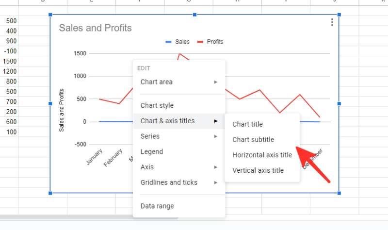
Step 3: Navigate to the Customize tab in the chart editor and select the option labeled Chart & axis titles.
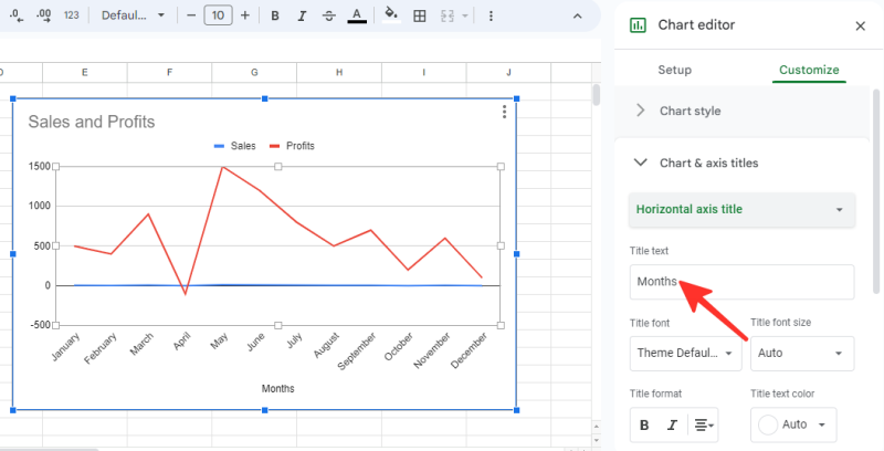
Step 4: Once you’ve opened the Chart & axis titles section from the Customize tab, you’ll be presented with various options to modify your axis titles. To change the title for the horizontal axis, simply select the Horizontal axis title from the list.

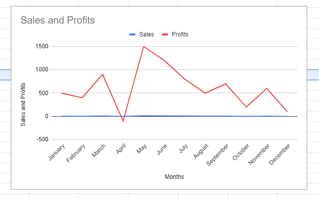
Step 5: Type in the desired label’s name under the “Title text” option. We are using ‘Months’ in the example below. You can also change the text format, font, font size, and color of the axis label.
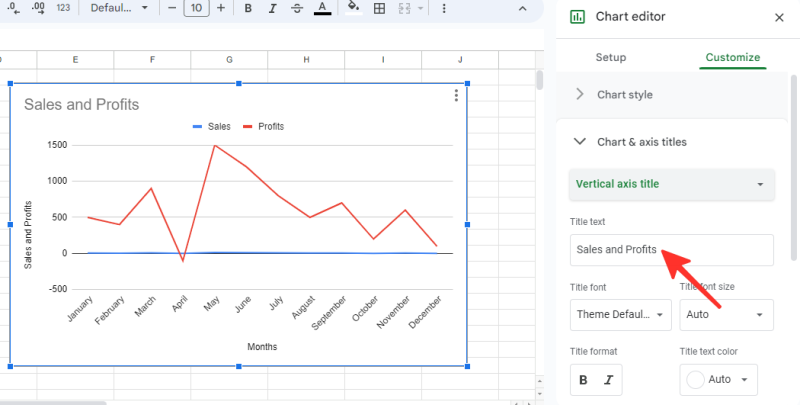
Step 6: To modify the title for the vertical axis, click on the Horizontal axis title dropdown button once more and select the Vertical axis title option from the list.

Step 7: Type the name of the label under the “Title text” option. We are using ‘Sales and Profits’ in the example below. You can also change the text format, font, font size, and color of the axis label.
Done. Your chart will now appear with the added and modified axis labels.
Tip: You can also modify the axis labels by right-clicking on the chart, selecting Chart & axis titles, and choosing the axis label that you want to change.
Add axis labels in the Google Sheets app on iPhone or Android using
Use the guide below to add vertical or horizontal axis label to your chart in a Google Sheets document easily using the official app on your iPhone or Android phone.
Step 1: Open the Google Sheets app on your phone.

Step 2: Open the Google Sheets file that contains the chart you want to add axis labels to.

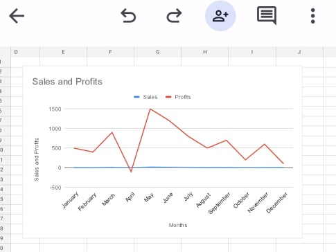
Step 3: Tap anywhere on the chart to select it.

Step 4: Click on the edit chart icon located next to the redo icon to add axis labels to the chart.

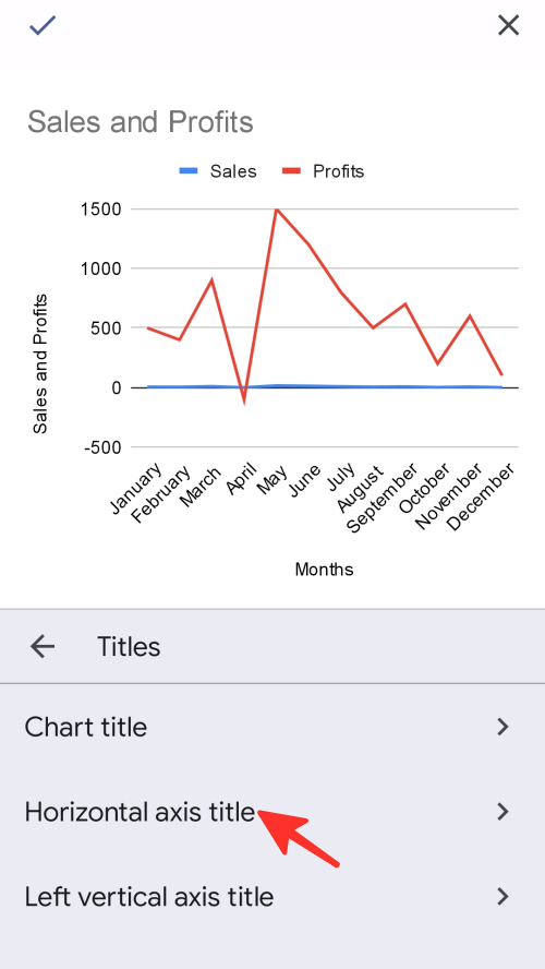
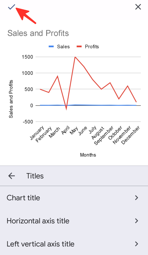
Step 5: Choose the Titles option from the list of available options.

Step 6: Select the Horizontal axis title option from the available list.
Step 7: In the pop-up window that appears, enter the preferred label name and click Update title to save changes. We are using ‘Months’ in the example below.

Step 8: Next, select the Left Vertical axis title option from the list of available choices.
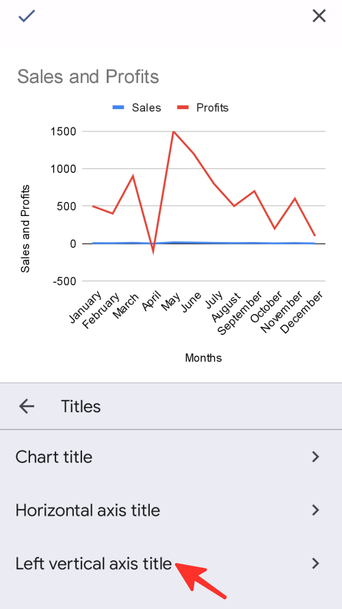
Step 9: In the pop-up window that appears, enter the preferred label name and click Update title to save changes. We are using ‘Sales and Profits’ in the example below.

Step 10: Click on the checkmark icon ✓ located on the left side of the page to save your changes.
That’s it! Your chart, along with the newly added axis labels, will appear on your screen.
Check out the step-by-step guidelines mentioned above on how to add axis labels in Google Sheets. You can use Google Sheets on your computer or phone, so pick the way that works best for you and get your work done!